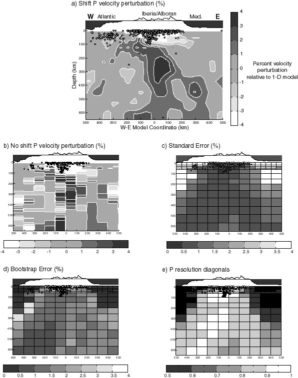
Figure 10. (Full color depth slices of these figures may be found
here). Cross sections showing an example section through the final 3-D P velocity model and the different attributes used to assess it. The cross sections are all located in the same position parallel and 25 km north of BB' along the southern coast of Spain (see Figure 8 for location of BB’). A topographic profile along the line of the cross section is shown for reference. (a) Final velocity model calculated using block shift-and-average approach (average of 100 separate inversions conducted with 10-km block shifts; see text for details). Anomalies shown are relative to the 1-D model shown in Table 2. Earthquakes (circles) are projected from a maximum distance of 50 km perpendicular to the section. The most striking feature is the high-velocity anomaly in the upper mantle. This anomaly reaches its shallowest point in the west where it is separated from the low-velocity region by the intermediate depth seismicity. (b) Result of a single inversion using the model parameterization shown in Figure 8 (no block shifting). The first-order features shown in Figure l0a, although more difficult to interpret, are visible. (c) Standard error in block velocities calculated using a posteriori covariance matrix. (d) Uncertainty in block velocities calculated using nonlinear bootstrap resampling. The high-velocity mantle anomalies are found to be of the order or greater than 2 times the bootstrap error (see Figure 10b), suggesting that they are robust features for this model parameterization. (e) Diagonal elements of the resolution matrix. High diagonal elements indicate strong control of observations on inversion result. Diagonal elements are higher in the west owing to the larger number of illuminating rays.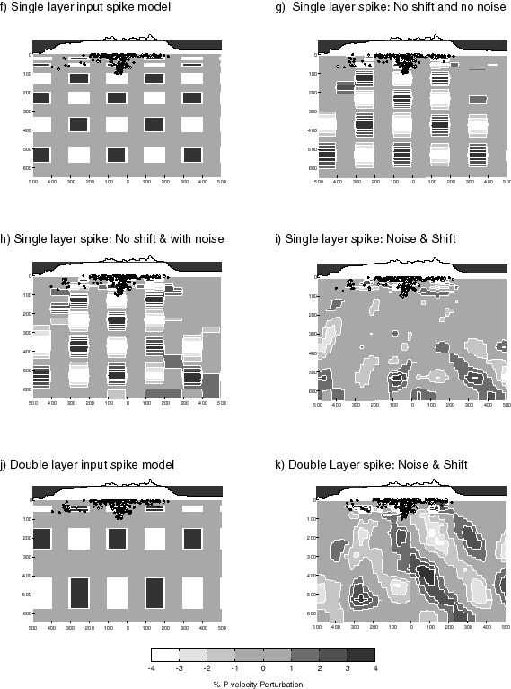
(f) Spike test input model. The 100-km blocks with ± 0.5 km/s perturbations relative to reference model were used, separated by a block with zero perturbation. A depth slice would also show a similar pattern of perturbations. (g) Result of inversion using synthetic arrival times calculated using spike model shown in Figure 10f. No noise was added to data and block boundaries used for inversion were coincident with the boundaries of the perturbations. Recovery is almost perfect in areas of illumination. (h) Identical to Figure 10g except representative Gaussian distributed noise was added to the data. The addition of noise degrades the recovery but not substantially. (i) Result of shift-and-average inversion with noise added to arrival times. Recovery is very poor throughout the upper mantle layers showing that degree of recovery of anomalies the size of a model block is strongly dependent on the model parameterization. Note the surprising recovery of velocity structure at the base of model (see text for discussion). (j) Modified synthetic model with spikes the same width as in Figure 10f but now extending over two layers with a two-layer vertical gap. Horizontal size and spacing of perturbations was not changed. (k) Shift-and-average recovery of spikes spanning two layers. Limited structure is now imaged in the mid-upper mantle but smearing is significant, indicating that depth resolution may be limited.